A Brief Look at Climate Models Developed by Skeptics

Bernie McCune

When Alarmists say “climate change is real!” I think yes it is, but “real . . . what?” My perhaps flippant answer to that question is real normal, real natural . . . among a few.  I think human caused climate change is real small.  These are some of the real issues that I want to explore here.

The first point is that the Intergovernmental Panel on Climate Change (UN IPCC) climate models are actually not real at all.  In fact based on the real data, they are turning out to be fairy tales.  Based on the real data, more realistic models are now being developed by very qualified groups and individuals. The improvement in modeling results over those by the IPCC appear to indicate that the billions of dollars spent by the UN IPCC and their modelers were completely wasted.

This independent and mostly unfunded modeling effort is being done by groups and individuals who can be characterized by their skepticism of IPCC modelers and climate alarmists.  In my opinion, alarmists include anyone claiming to be alarmed by what they imagine to be a dramatic rise in global temperatures due to human activities.

The skeptical modelers are showing us a more realistic view of past present and future climate change that follows mostly natural temperature patterns.  All of these skeptical models indicate a more benign climate outcome.  In every case they are able to bound the problem of cause and effect so that they are beginning to dramatically reduce the wide uncertainty range of expected global temperature increase due to atmospheric CO₂ concentration.  Under the research guidance of the IPCC this uncertainty has remained in the 1.5° C to 4.5° C range for the past 30 years.  In the United States, the Environmental Protection Agency has arbitrarily and without any scientific basis decided to be more conservative by increasing the upper bound of uncertainty to 10° C.

On May 20, 2017, I gave a presentation to our small Las Cruces, NM atmospheric group titled Some Models Based on Natural Cycles Versus the Failed IPCC Models.  On the title page I quoted Fred Singer “Before facing major surgery, wouldn’t you want a second opinion? When a nation faces an important decision that risks its economic future, or perhaps the fate of the ecology, it should do the same.”

Model Basis

IPCC Models are based on a feedback theory of warming caused mainly by CO₂ as it affects water vapor using complex parameterizations.  There are now a number of simple models that use real data from nature to show various lengths of cyclical patterns having both warming and cooling elements to the cycles.  Over the past couple of decades the IPCC models that use CO₂ as a basis for warming, project a continuing warming trend that is not reflected in the actual temperature data plots as seen below.

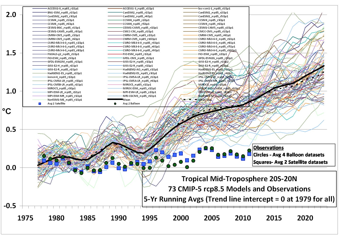
Note above that the average of all the IPCC models (bold black line) has dramatically diverged over the past 20 years from the real data shown by blue squares (average of two different satellite datasets) and black circles (average of 4 balloon datasets).

The basis of the IPCC view of human-caused climate change is the theory that human-produced atmospheric CO₂ is the cause of catastrophic global temperature rise.  Not only is the theory that all combined sources of atmospheric CO₂ are causing catastrophic warming proving to be grossly overstated, but also the theory of human-produced CO₂ warming (a subset) is likely to be of little consequence.

A growing body of data indicates that sensitivity to warming from a doubling of concentration of CO₂ in the atmosphere is likely to be less than 1° C.  Richard Lindzen questions the negligible effect of any non water based greenhouse gases (GHGs) that might cause an increase of a few watts per square meter when atmospheric moisture can decrease incoming solar energy by at least 100 watts per square meter or more — a case of classic negative feed back. 

David Evan makes a Simple Comparison

Dr. David Evans did an extensive but simple analysis of basically the feedback theory of the IPCC group and showed it to be overstated based on actual data. There is a several page report that goes into the detail of his analysis but the results are cleanly captured in the next figure. The most recent IPCC reports and the skeptics can probably agree for the sake of argument that direct effects of CO₂ doubling is only 1.1° C. The inflated feedback amplification factor is used by the IPCC to distort the effects. David Evan indicates and can show that the feedback factor is less than 1.

At then end of this report, another skeptic modeling team also shows that feedback effects inflated by the warmists are scientifically indefensible.

There is a simple common sense view that explains the effects of atmospheric moisture that supports moisture feedbacks of 0.5 or less.  It is true that with cloud cover at night here in the desert SW especially in the winter, we find that surface temperatures for brief periods tend to be warmer.  Even with present “high” atmospheric CO₂ concentrations at night here in Las Cruces, surface temperatures plummet when there is little or no moisture in our atmosphere.  In the daytime; however, clouds and moisture have multiple times the effect on reducing surface temperatures than CO₂ does on increasing surface temperatures.

New Models based on Data

Over the past couple of decades the analysis of long term data has shown that there are natural cycles that apparently drive surface and ocean temperature variations.  None of these variations show any long term warming trends.  They actually cycle over a variety of periods.  Three cycles seem to have now emerged from what had seemed to be a chaotic, un-patterned temperature record.

The periods of these three cycles generally follow about 1000-year, about 200-year, and about 60-year cycles. For near term correlation (100s of years of temperature evidence), these cycles as they interact with each other tend to follow the actual temperature variations found in data from the past.  Our own group members have recognized the 60- and 1000-year patterns.  A clear solar 200-year pattern also exists.

It seems obvious that the sun drives all these patterns in some direct and indirect ways.

We have already seen Dr. Evan’s Alarmist versus Skeptic view of how the climate seems to work.  The IPCC models seem to now be running hot due to incorrect feedback factors put into those models.

The Elephant in the Room

We know from geologic and ice core records that there are longer term (100K year) deep glacial periods of very cold climate change.  These glacial periods can be clearly seen in past proxy data.  Even though I am not exploring these huge climate change events in this discussion, the question arises – what causes them and why for the past million years have they occurred like clock work?

Glacial ice ages lasting about 100 K years and short inter-glacial warm periods lasting about 8k to 11k years can be clearly seen in the geological record.  Why are these deep glacial periods 10 to 20 deg C colder?  And the big questions!  Is the next one now on its way?  Could the next ice age begin to emerge in the next couple of hundred years or less?

Some Reasons Why IPCC and Skeptic Models Do Not Agree

Alarmists note that an increase of atmospheric CO₂ (about 120 ppm) in the past almost 80 years is causing an increase in global temperature. Skeptics mostly agree that there may be some increase but the data shows only about 0.6 to 0.8° C increase from all causes in that period. With a doubling of CO₂ in the next 60 years (by 2077), alarmists claim that temperatures could increase from somewhere between 2 to 8 degrees C.

First of all, it is not clear that this doubling will occur that quickly.  According to present rates of atmospheric CO₂ increase, the doubling will actually occur around 2160.

Secondly, this rapid increase in human-produced CO₂ during the next 60 years has the annual rate of CO₂ entering the atmosphere at rates as high as 5.5 ppm/yr, and causing global temperatures to rapidly rise.

The data, so far, does not support their theory.  The annual rate of CO₂ increase over the past several decades basically has averaged less than 2 ppm/yr, and global temperatures are clearly not increasing at the rate that their IPCC models predict.  These modest annual increases of atmospheric CO₂ (less than 2 ppm/yr) occur in spite of a very huge increase in human produced CO₂.

In 1972 annual estimated total global human-produced CO₂ was about 5 gigatonnes.  That same year the increase in concentration was about 1 ppm.  In the past 20 years an average of 2 ppm rate of increase continued in spite of the fact that from 1997 there were 22 gigatonnes of CO₂ produced to the present where 32 gigatonnes were produced (an increase of 10 gigatonnes).

All large annual increases of atmospheric CO₂ for the past 30 years (such as those in the realm of 3ppm/yr) were caused by naturally occuring El Ninos.  So what does human produced CO₂ have to do with it?  Mostly nada?

I will next showcase four additional models that have been developed over the past decade.  There are two done by individuals – Dr. Girma Orsengo and Ed Caryl.  Caryl’s model uses all three cycles noted above.  Then there is an ex-NASA team from Houston calling themselves “The Right Climate Stuff (TRCS)” who use the 170 year thermometer dataset that shows a 60 year pattern in it.  Finally, Lord Monckton’s team uses the IPCC equations and theory but substitutes different input values based on some in depth analysis to show that temperatures are not going to rise at anywhere near the alarming rates projected by the IPCC models.

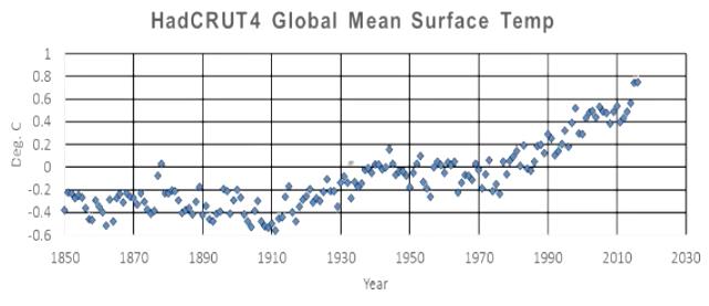
The following graphic shows a commonly used temperature dataset that goes back to 1850 produced by the UK Met Office – HADCrut.

This data set is generally accepted by all researchers in the climate research field and is noted by each of the modelers who use it to make their case throughout the rest of this report.  I modified the above graphic with hand annotations to show a global 60-year AMO cycle that I found earlier in the New Mexico temperature data when Michael Mann and his hockey stick made me wonder whether NM temperatures were warming.  There was some warming in NM urban areas but cooling in NM rural areas, but that is another story.

I have included in the below plot a very recent temperature data set from a modern US group of sites called the US Climate Reference Network (USCRN).

Since this data set was only available from January 2005 until May 2015, it compliments and adds to the “flat” data record of the recent past that is shown by real satellite and balloon data in the very first graphic of this report.  The USCRN is a very new system of monitoring stations and this data set is all we have right now for an extensive rural US climate network. This is not a global record but it certainly indicates that at least the rural sites in the continental US plus Alaska and Hawaii are not following any sort of global warming trend (with no chance of an Urban Heat Island –UHI- effect). In fact if you look closely, the trendline has a slight negative tilt.

The Girma Orssengo Model

The first actual model to be reviewed was done by an individual, Dr. Girma Orssengo, using all IPCC based data and smoothed sine wave projections to show what we might expect in the future. He presented this almost 10 years ago, and it was not very well received.  I really liked the simplicity and the idea of using a known 60-year ocean based cycle.  He uses a sine wave to bound the HadCRUT data and project it to 2100.  When I found a recurring pattern in the NM data, I was able to fit the data to a smooth sine curve which turned out to be the AMO.  I hand drew a continuation of the model in order to reach my projected point of CO₂ doubling in 2160.

There is a more in depth discussion of Girma Orssengo’s model here, but this single, simple graphic and simple idea of a natural cycle model in this snapshot is all you really need.

Study it a little to see the HadCRUT data that is used to verify his sine wave plot.  Look at the Global Mean Temperature Anomaly (GMTA) equation.  If you agree that this is a reasonable model, look at what the temperature in 2100 is likely to be (0.63 degree warmer than what it was in 1965). Look at the IPCC alarming projection and remember what the USCRN data set is showing us. And note that if Orssengo is right, there is nothing very alarming even in 2200 where the temperature is expected to be 1.1 degrees warmer than 1965.  His model predicts cooling over the next couple of decades to almost what temperatures were in 1965.

This is one person’s effort using a well known 60-year temperature pattern that is natural and has been cycling this way for 100s of years.  So far, the HadCRUT data set is mostly bounded by his model envelop. The bright blue and red excursions are what we call weather but this climate model over the past 130 years is on track to be a completely valid if very simple model.

The Caryl Model

Ed Caryl is another individual who has produced a more complex model that is still based on all three of the natural cycles we have previously discussed (62, 204 & 1040). These are known cycles with the 62-year cycle pattern that is similar to El Nino Southern Oscillation (ENSO) related cycles of the Pacific Decadal Oscillation PDO and the Atlantic Multi-decadal Oscillation (AMO).  The 200-year cycle relates to solar activity that can be measured by Carbon 14 levels in the atmosphere.  The 1000-year cycle relates to the Bond cycle that can be clearly seen in ice core samples.

Caryl aligns the three cycles and blends them into both a noisy and smooth pattern.  The alignment relates to the phase of the cycle such that it is lined up with actual patterns of real data in the past so that they can be projected into the future to predict what actual temperatures might really be in the next couple of hundred years.

We are now in a peak of the 1000-year Bond cycle.  The 60-year cycle has peaked and is now cooling and so has the 200-year cycle.  With all three cycles starting to cool together, perhaps Girma’s model is correct in suggesting that the next few decades will be cooler.

The next graphic shows a plot of the sum of all three curves.  The period is from 1000 AD until 2200 AD so it includes the thermometer record of recent time.

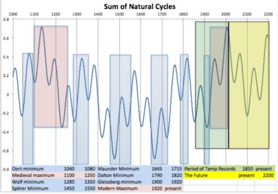
What is of great interest to me is that Caryl’s model does a very good job of hindcasting periods of sunspot activity and temperature cooling and warming as noted by the blue and pink boxes.

This model suggest that for the next 100 years we will be entering a cooling period. And the next zoomed in part of the above graphic superimposes the HadCRUT data onto the plot of Caryl’s model to again (just like in Girma’s model) show that the Caryl Model bounds real thermometer data to an even better degree than Girma’s did.

Caryl’s smooth clean plots don’t look like the real HadCRUT data so he developed a more noisy chaotic plot of his monthly stepped data using a method of random numbers and produced the plot below of the previous 1000 years.

Zoom in on the last 214 years, which easily cover the HadCRUT thermometer record. Then just eyeball it with the actual HadCRUT plots that I have scattered all through the first part of this report.

It seems even to replicate some of the well known El Nino warm spikes and it certainly follows general trends in the thermometer record.

Now there is one last one to see what the future might bring.

Caryl supplied all his model imputs in spreadsheet form so that anyone can look at and play with them.

The “Right Climate Stuff” Model

An informal group of experience ex-NASA engineers and scientists in Houston started meeting in a restaurant to discuss the issues that were being raised by climate change.  This is very much like our group here in Las Cruces where we meet on the third Saturday of each month for brunch and discussion.

In the case of The Right Climate Stuff (TRCS) team, Dr. Harold Doiron has become the spokesperson for the group. He has an hour long presentation on the material that I will briefly discsuss here.

Both of our groups started to discuss and complained about the many failings of the IPCC un-validated models, but the TRCS team went on to develop their own model, and surprise – surprise, their first graphic looks very familiar.  We see later in this part of the report how this fits into their model, but first let’s look at the complaints.

Issues between TRCS Team and IPCC

The main point of disagreement between TRCS and IPCC related to the unrealistic IPCC Equilibrium Climate Sensitivity (ECS) and Transient Climate Response (TCR) metrics.   Consequently, the Team developed their own Transient Climate Sensitivity (TCS) metric that was comparable to the real data.

Another major issue that all skeptics have with the IPCC models and a key one for the TRCS team is the fact that the IPCC models have not been validated.

Finally, the Team disagreed with the idea that a 0.8 deg C warming over the past 165 years should be something to be alarmed about.

ECS value is an academic rather than realistic concept that tracks long term climate effects, and TCR is dramatically over-estimated by IPCC models.

ECS is defined as a global temperature rise that occurs with a doubling of atmospheric CO₂ from pre-industrial levels to about 560 ppm.  After 30 years, the IPCC Assessment Reports continue to show ECS values of wide uncertainty ranging from 1.5 to 4.5 deg C.

One of my major gripes and for the TRCS team also is that the EPA arbitrarily uses an even wider range of ECS from 1 to 10 deg C for regulatory purposes.

Defining the Terms and Building the Model

Trenberth’s simplified radiation balance diagram is the beginning of the process to discover climate issues and to start the dialog among dissenting parties.  For the TRCS team there is basic agreement on most of this diagram.

The Team decided to look at the earth space thermal problem as more like a spacecraft with which they were much more familiar, and they already had the math and physics to deal with it.

What the climate scientists had with the above process was an unbounded complicated thermal nightmare.  One of the variables was a changing emissivity due to water in all its forms.  By getting a handle on the terms involving emissivity the rest of the problems could be solved.

W= Water Vapor C= Carbon GHG G= Other GHG T= Temperature (288 K)

β= GHG Effects a= albedo S= incoming radiation (341.3 W/m₂)

e= emissivity – average earth (238.5/(σT₄) = 0.611) Q= energy into oceans (0.9 W/m₂)

OLR = eσT₄ = 238.5 W/m₂ σ= 5.67(10)_–8W/m₂/K₄

Emissivity Constant= 4eσT₃ = 1/0.302

Radiative Forcing since 1850 (Computed from CO₂ IR absorbtion bands) = 3.71 W/m² (assumes 284.7 ppm)

Most people agree in general terms with most of these values and with the way they interact.

TRCS team looked at the earth as a spacecraft with the atmospheric skin and surface of the earth much like that of an actual spacecraft skin.  By collecting all the elements and terms the Team began to look at all of them and then build some mathematical functions that had familiar relationships.

The issue of refining the broad uncertainties in the ECS was where Dr. Doiron stopped and made the comment that climate scientists had gone open loop and had lost their way. “They needed some adult supervision,” and clearly the IPCC were not in a position to offer any of that.

In order to get past the ECS and TCR issues that they had with the IPCC methodology they began to develop their own way to look at the problem.

So the next step was to look at the data and see if they could use it to bound the TCS value. They began the process by using HadCRUT data.

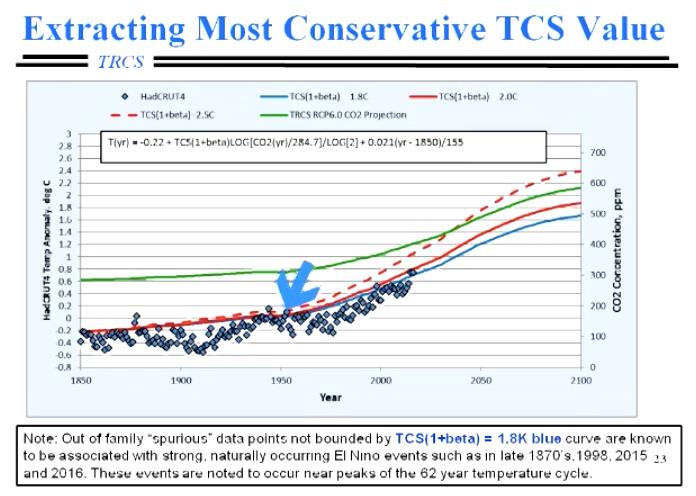
What at first seemed to be outliers became “warm” El Nino year data points.  So rather than bounding these naturally occurring temperature spikes they left them alone with the knowledge that they could not be caused by humans or any sort of CO₂.

The next task was to determine the worst case future warming that could be caused by CO₂.  One member of the team determined what the value of atmospheric CO₂ would be if all known carbon sources were burned.  The value happens to be a large fraction of what a doubling of atmospheric CO₂ would be at sometime during the next century.  A bounded value of TCS could be estimated so that the model equations could be solved.

The graphic below shows a set of possibilities.  The maximum temperature rise is noted to be 1.2 K before all fossil fuels known are burned up which is the bounded value of TCS.

The final derivation of TCS is shown in the next graphic.

With all the terms bounded, TRCS team were able to narrow the uncertainties.

This is a very incomplete handling of a much more complicated model.  This model assumes a much more benign effect from a doubling of CO₂.  The previous models that were discussed do not pay much attention to CO₂ while at the same time, they see these same very small effects.

TRCS team members are very interested in validating their model and are looking for a team to do the honors.  They highly recommend that the IPCC models be treated in the same way and as soon as possible.

Monckton Versus the IPCC

The last team that produced a model included Lord Monckton. They had a number of bones to pick with the IPCC.  A major issue for this team was to actually find a method to model the feedback that the IPCC was assuming was quite large (see the beginning of this report and David Evan’s work).

The assumption that temperature feedbacks will double or triple direct warming is unsound.  In fact, feedbacks may well reduce warming, not amplify it.  The Bode system-gain equation “models” the mutual amplification of feedbacks in electronic circuits, but when models erroneously apply it to the essentially thermostatic climate on the assumption of strongly net-amplifying feedbacks, its use leads to substantial overestimation of global warming.

The equation for feedbacks is well known and accepted by all parties involved in this discussion.

There are some issues with factors on the left side of the graphic above, but the big issue with all the skeptics is the part of the equation on the right side of the page which contains the feedback factor.

Climate modelers have failed to cut their central estimate of global warming in line with a new, lower estimate of the feedback sum (AR5, fig. 9.43). They still predict 3.3 K warming per CO₂ doubling, when on this ground alone they should only predict 2.25 K of which direct warming and feedbacks each contribute about 50 %.

There are some fundamental laws of feedback that need to be reviewed as well as issues of stability and how the FB systems actually work.

The central value of temperature being 2.25 K is most likely to be correct in order for all other factors to remain within a reasonable boundary and for the system to have any chance of being stable.

Then the issue becomes what is the actual value of feedback.  Monckton shows that the IPCC scientists have made a mistake about the nature of the inputs and outputs and therefore have come up with the wrong value for the feedback.

The following graphic uses absolute values of temperatures, and, therefore, comes up with a value of feedback that is about 0.005, a very small value.

The IPCC scientists do it wrong by using inputs and outputs that are deltas (not absolute values) with the following result.  A feedback value that is 2 orders of magnitude too large.

So with a rigorous mathematical proof of the feedback now shown, most of the climate experts in feedback theory (there are not many of them) seem to now agree that the FB issue has been handled incorrectly by the IPCC scientists, and that this team has proven it.

So the final result gives an ECS that almost all other skeptics have intuitively found.  This is a fairly solid proof of it with this final graphic as the result.

Some Final Issues from the Monckton Team

Though general-circulation models suggest that 0.6 K man-made warming is “in the pipeline” even if CO₂ emissions cease, the simple model, supported by almost two decades without significant global warming, suggests that this is not the case.  In other words, there is no committed but unrealized man-made warming still to come.  The TRCS team came to a similar conclusion.

AR5’s extreme RCP 8.5 forcing scenario predicting ~12 K anthropogenic warming, is unjustifiable.  It was based on CO₂ concentration growing at 5.5 ppmv per year this century, while AR4’s central estimate was below 3.5 ppmv per year, and the current growth rate is little more than 2 ppmv per year.
  Again, several of us have come to this same conclusion.

Monckton’s model does not even address the natural (data driven) process to any extent. He admits this (see his presentation) and that there are issues of naturally driven climate change that are real.  The feedback model simply shows where the IPCC models fail.  It addresses areas where we have complained about the IPCC and warmist’s assumptions in the past (eg. annual increase of CO₂ greater than 2 ppm, positive rather than negative feedback etc.)

My Report Conclusions

The complex IPCC models using hypothetical constructs for most of their parameters do not come anywhere near what we see real global temperatures doing.  As demonstrated in this post, there are several simple almost homemade models that are doing a much better job of following actual temperatures for the past few decades and that have some credibility in helping us predict future temperatures with much greater certainty.