
by Bernie McCune
This whole discussion began with a posting on Watts Up With That by Hartmut Hoecht posted on July 11, 2018.

It is worth reading the whole thing but I will summarize it here. Various ways of measuring ocean temperatures from long ago until present times are discussed and questions of uncertainty and errors are raised. Recent and even very old reports on sea surface temperature (SST) values are often given in fractions of a degree. In reality, until very recently, the collection process had obvious errors that were greater than one degree.
Cooling periods in the SST records seen in the 1940s and 1970s of 0.3º C were noted in the data with some concern about collection methods but this period is known to be a AMO[efn_note]Atlantic Multi-Decadal Oscillation (AMO) is a climate cycle index that has a roughly 60 year period. The natural variation of the average sea surface temperature of the North Atlantic Ocean basin from the equator to 80o N is used to produce this index.[/efn_note] (and with less influence PDO[efn_note]Pacific Decadal Oscillation (PDO) is another climate cycle index that also has about a 60 year period. It is related to the El Nino Southern Oscillation (ENSO) and is a robust, recurring pattern of ocean-atmosphere climate variability centered over the mid-latitude Pacific basin. The PDO is detected as warm or cool surface waters in the Pacific Ocean, north of 20°N. It was named by biologist Steven R. Hare in 1997 when he noticed it while studying salmon production pattern results in the North Pacific Ocean. This climate pattern also affects coastal sea and continental surface air temperatures from Alaska to California.[/efn_note]) 30 year cooling period. In order to discern these 0.3º C changes in the data, instruments with an accuracy of 0.1º C must be used. The rule of thumb noted that the instrument must have better than three times the accuracy of the targeted resolution. Instrument errors of 0.5 to 1º C were the norm until the 1980s but continued into the 1990s as modern instruments finally replaced all the old ones.
Temperature data collection out in nature focuses not just on the thermal reading device by itself. There is always a process, which comprises the data collection method, temporary data storage, data conversion and transmission, manipulation, etc. Add to this the variations of time, location, protocol, sensor drift and sensor deterioration, variations in the measured medium, different observers and interpreters, etc. All of this contributes to the system error. The individual error components are separated into the fixed known errors and the random variable errors. Further, we must pay attention to the “significant figures” when assessing error contributors, since a false precision may creep in, when calculating total error.
This WUWT discussion goes on to explore methods using wooden, canvas and modern metal buckets and scoops as well the various floats and buoys used in the 1990s until present. There were a host of issues that related to the collection methods and tools along with the other error components noted in the previous paragraph. It is worth reading and studying to realize that many folks using historical and even fairly recent ocean temperature data have failed to properly understand systematic error conditions and to properly present their findings with these considerations in mind. There is a lot more detail in the actual report.
I then did some more research on systematic error studies and techniques and found an essay by Pat Frank that he presented in Sicily in August 2015. He reported in WUWT in April 2016 which can be found here:
I want to give a much more in depth discussion of this information in the rest of this report. This discussion will explore systematic errors (SE) in measuring all types of long term climate temperature both in the ocean and the atmosphere. These SE enter into the experimental and observational results through uncontrolled and often cryptic deterministic processes[1]. These error processes start with the most basic one, which is consistent operator error. Another is error from uncontrolled experimental variables. Then there is instrumental inaccuracy including levels of malfunction and lack of calibration. Uncontrolled variables can impact the magnitude of the measurement and/or completely change the course of the experiment. These various SEs are difficult to detect and remove.
The author offered a real experimental laboratory case of titration of dissolved ferrous iron that was contaminated by a trace amount of air to produce results that closely follow a real uncontaminated titration[2,3].
This is a case of inadvertent entry of a trace of air that was enough to completely change the course of the experiment.

The left hand plot with erroneous data seems to be accurate and follows a trajectory (inset) completely consistent with equilibrium thermodynamics. It looks like it is valid and the data are convincing, but wrong. Contaminated experimental or observational results can look and behave just like good data, and can rigorously follow valid physical theory.
Systematic error is difficult to detect and remove. Methods of elimination include careful protocol control and instrumental calibration under conditions identical to the observation or experiment.
Another example is of dramatically reducing clock error in a highly accurate atomic clock by elimination of black body thermal noise produced by the sensor itself[4].
The timing element is a cluster of fluorescing Strontium atoms trapped in an optical lattice. Thermal noise is removed using data produced by a sensor that measures the black-body temperature of the instrument.

In the 1960s when I was using quartz and rubidium based atomic clocks to assist in obtaining precise navigation positions from Navy navigational satellites the best timing accuracy available was tens of microseconds (10-6).
By a whole process of finding and removing systematic errors over many decades we have attained the present incredible level of timing precision.
Principles of Removing Systematic Error
Systematic error cannot be averaged away using repeated measurements. Repetition often increases the error. A very basic principle when systematic error cannot be eliminated and is known to be present, is to fully report it along with the data. The most basic idea in all measurement practices is to be very sensitive to the fact that systematic error is likely to occur and must be accounted for. Modifying or massaging data will likely exacerbate systematic errors. Characterization of the data using clear systematic error detection and presentation methods is probably the only allowable limit to data management that should be accepted.
In graphical presentation of measurement or data calculations, systematic error should be represented using uncertainty bars[1]. These uncertainty bars communicate the reliability of the result.
Systematic Errors and Air Temperature Instrumentation
During the last half of the 18th century and most of the 19th century, land surface air temperatures were measured using liquid-in-glass (LiG) thermometers. During most of the 19th century a series of different housings were also used. Until about 1985 the housing was a Stevenson screen also known as a Cotton regional shelter (CRS) [5,6].
After 1985 thermistors or Platinum Resistance Thermometers (PRT) housed in an un-aspirated (no fan) cylindrical plastic shield replaced the CRS/LiG thermometers in most areas of the globe. In 2000 the US Climate Research Network (USCRN) deployed sensors with a trio of PRTs in separate aspirated shields[5,7-9]. This system is a very radical change for air temperature measurement and warrants a detail description.
Each USCRN station has three thermometers which report independent temperature measurements each hour. These three observed temperature values are used to derive a single official USCRN temperature value for the hour. This single value is sometimes a median and sometimes an average of various combinations of the three observed values, depending on information about which instruments agree in a pairwise comparison within 0.3°C. Each station transmits the three independent observed values; the computation of the official USCRN temperature value is done after these values arrive at NCEI. The discussion below describes the details of the three observed values.
Each station has three Thermometrics Platinum Resistance Thermometers (PRT), each of which is housed in its own Met One 076B 7308 aspirated solar shield. Each thermometer measures the temperature (in degrees Celsius) every 2 seconds. Every 5 minutes the station data logger computes the average of these 2-second values, giving 12 5-minute averages for each thermometer. Standard deviations are also calculated for each thermometer. Finally, a moving 5-minute average displaced 10-seconds at a time is used to determine the maximum and minimum 5-minute periods ending within the hour in question.
In addition to the thermometer values, the station also measures the speed of the fan in each aspirated shield. As the shield’s fan rotates, a contact closes and generates a pulse twice per rotation. The data logger counts these pulses every two seconds. Every hour these 2-second values are averaged to obtain an average number of pulses per second for the hour.
The hourly data stream from the station thus include the average pulse rate per second for each of the three sensors. The actual speed of the fan in revolutions per second is half the pulse rate.
Air Temperature Measurement Error
Clearly the USCRN temperature measurement systems have made some huge steps to decrease systematic errors. For almost the whole of the previous almost 200 years, data gathering techniques must be considered to be quite antiquated. Error issues for that whole period of an increasingly wide spread weather data temperature measurement system has to be discussed.
Un-aspirated air sensors rely on the prevailing wind for ventilation and it is known that systematic error occurs when air movement is less than 5 meters/second [9,11]. Solar irradiance can heat the sensor shield, warming the interior atmosphere around the sensor. Albedo effects that vary from grass to snow surfaces, not to mention pavement and concrete surfaces, can lead to a warm bias. It is a well known systematic error value when urban temperature measurement sites are tightly encroached on by various human types of heat sources that produce urban heat island effects. These alone can cause several degrees of warm bias.
Calibration and Instrument Error
For a majority of the time that global temperatures were being measured (about 135 years), it was very difficult to determine the precision and accuracy of the LiG readings being taken. Since very little was done during that period to calibrate and cross check instruments, error values can only be guessed at. A fairly recent calibration experiment must make us seriously question the value of all the air temperature data taken until the USCRN stations were established.
This calibration experiment in 2007 and 2008 was conducted on the Alpine Plaine Morte Glacier in Switzerland by Huwald, et al[12]. This experiment tested the field accuracy of the RM Young PRT (platinum resistance thermometer) instrument housed in an un-aspirated louvered shield, situated over a snow-covered surface.


Temperature trends were recorded simultaneously where the red plot is the RM Young PRT instrument and the blue plot is the sonic anemometer. The RM Young instrument showed a significantly warmer winter air temperature trend.
The slope of the RM Young temperature is 3 times greater than the slope of the sonic anemometer. The significance of this experiment is that this type of Young instrument is similar in design and response of advanced probes being used on a world-wide basis since about 1985. So this data referenced to a common mean will show a spurious warming trend even considering that it is a modern global temperature average.
This warming systematic error is characterized in the following graphic where day time errors average 2.0º +/- 1.4º C while night time errors averages 0.03º +/- 0.32º C.The systematic errors for this modern instrument when no independent calibration instrument is available for any given daily mean temperature show an associated 1 sigma uncertainty of 1º +/- 1.4º C. 
From the above histogram it can be clearly seen that the uncertainty is not random nor is it constant. It cannot be removed by averaging individual measurements or by taking anomalies. And subtracting the average bias will not remove the non-normal 1 sigma uncertainty. Entry of these specific station temperature records into the global average will carry the average error along with it.
Before inclusion in a global average, temperature series from individual meteorological stations are subjected to statistical tests for data quality[13]. Air temperatures are known to show correlation R=0.5 over distances of about 1200 km[14,15]. The first quality control test for any given station record includes a statistical check for correlation with temperature series among near-by stations.
The following figure shows that the RM Young error-contaminated temperature series will pass this most basic quality control test. Furthermore, the erroneous RM Young record will pass every single statistical test used for  the quality control of meteorological station temperature records worldwide[16,17]. The inset[14] is very blurry but it shows correlation of temperature records from meteorological stations in the terrestrial 65-70º N, 0-5º E grid. The 0.5 correlation length is 1400 km.
Another calibration experiment was carried out at the University of Nebraska, Lincoln[11] with a variety of screens that held identical HMP45C PRT sensors. An aspirated RM Young PRT probe rated as accurate to less than +/-0.2º C was used as the calibration reference.
The figure below shows the average systematic error of the HMP45C PRT probe[10,11,18] in an MMTS labeled E in the above photo with the calibration RM Young reference labeled G in the above photo. The top graph is a Spring-Autumn test over grass and the bottom is a Winter test over snow[10]. The shield labeled F in the above photo is an old fashioned CRS.

The average annual systematic uncertainty produced by the MMTS shield can be estimated from these data as, 1 sigma = 0.32 +/-0.23º C. The skewed warm-bias distribution error over snow is similar in magnitude to the un-aspirated RM Young shield in the Swiss experiment.
CRS shelter is at least as accurate as a traditional LiG thermometer. The warm bias in the data is apparent, as is the non-normal distribution error.
The next plot shows the average systematic measurement error produced by a PRT probe inside a traditional CRS shield[11].

The average day-night 1 sigma value = 0.44º +/- 0.41º C of systematic measurement error produced by a PRT temperature probe in a traditional CRS shelter.
So considering reasonable bounding condition, the PRT/CRS experiment can be used to estimate a lower limit of systematic measurement uncertainty found in the land-surface temperature record covering all of the 19th century and most of the 20th century[19,20].
Sea-Surface Temperature
A lot of effort has gone into understanding sea surface temperatures (SST)[21-28], but there have been very few field calibration experiments on the sensors that were used. Bucket and ship intake cooling water measurements using a variety of LiG thermometers was carried out from the beginning until the mid-20th century.
Ben Franklin and his cousin Timothy Folger who was a whaling captain characterized the Gulf Stream and made a map of it that was first printed in London in 1769. He apparently recorded temperatures from  thermometers that were dragged in the water. This method could not give very precise values of SSTs but certainly could characterize the depth and width of the Gulf Stream (up to 10 miles wide and about 3 feet thick) and give rough values of temperature differentials. The map showed it’s location in the Atlantic to a degree that compares very favorably to present day maps.
Growing use of electronic sensors since 1980 on drifting and moored buoys have become increasingly important in SST measurements and calibration studies have focused on them[29]. A series of experiments
reported by Charles Brooks in 1926 were the most comprehensive field calibrations done on bucket and engine-intake thermometer SST measurements[30].

Systematic measurement error in engine-intake (left side in red) and bucket (right side in blue) SSTs as reported by Brooks.
Brooks recruited a ship’s officer to monitor the ship board measurements after he finished the experiments and had departed the ship. Errors after he departed were about twice as large as they were when he was aboard. Care in making measurements obviously deteriorated perhaps “back to normal”. Standard assumptions in the field before this was that temperature sensor errors are constant for each ship.
Later SST Error Studies
In 1963 Saur reported on the largest field calibration experiment of engine- intake thermometers that was carried out by volunteers aboard 3 US military transport ships and 9 US Navy Radar Picket ships during 92 different trips on the US central Pacific coast[31]. The experiment included 6826 pairs of observations.
These results were combined to give similar measures for each ship (ship bias and standard deviation) and estimates of these measures for a large number of ships (fleet). Reported sea water (injection) temperature observations vary considerably in quality. The fleet bias, or mean difference, of injection temperature observations as compared to surface temperature observations is estimated to be 1.2º±0.6º F and the standard deviation of differences to be 1.6º F. Among the 12 ships, the ship bias, or mean of all differences derived from observations of a given ship, ranged from 0.5º F to 3.0º F, which is probably due to variations of the thermometer accuracy and of the thermometer installations between ships. The standard deviation about these means was 1.3º F, which is a measure of the variability of present data records, provided that the bias for each ship could be determined and a correction applied.The variability of differences in the observations from a single ship is attributed to the system of taking and reporting sea water temperature observations from an injection thermometer. To improve the reliability of reported sea water temperature observations, a change to an electrical resistance or thermistor thermometer, specially designed and installed to measure the sea water temperature and having a remote indicator on the ship’s bridge, is recommended. If this change were made, it is estimated from trip data that the standard deviation of differences would be reduced to less than 1.0º F.
Systematic error results in recorded engine-intake temperatures aboard one of the military transports operating from June-July 1959 are shown in the next figure. The mean systematic bias and uncertainty represented by the data are, 1 sigma = 0.9º +/- 0.6º C which are comparable with Brooks’ values. 
Saur’s Report (1963) . . . using the above figure “as a typical distribution of differences” reported for all the various ships included in the study and being compatible with those values reported by Brooks. And in conclusion he noted that . . .”the average bias of reported sea water temperatures as compared to sea surface temperatures with 95% confidence limits, is estimated to be 1.2º +/- 0.6 F [0.67º +/- 0.35º C] on the basis of a sample of 12 ships. The standard deviation of differences (between ships) is estimated to be 1.6º F [0.9º C]. Thus without improved quality control, the sea temperature data reported currently and in the past are for the most part adequate only for general climatological studies”.
Mid to Late 20th Century SST Platforms – BT and XBT
Measurements from bathythermograph (BT) and expendable bathythermograph (XBT) instruments have made significant contributions to the SST record[32]. Very early BT instruments pre-date WW2.

Large numbers of records began to appear after the war and really taking off in the 1950s. Extensive BT and XBT calibration experiments revealed multiple sources of systematic error mostly from mechanical problems and calibration errors[33-35]. Field BT measurements exhibited 1 sigma = 0.34º +/- 0.43º C errors[35] which is more than twice as large as the manufacturer-stated accuracy of +/- 0.2º C and reflects the impact of uncontrolled field variables.

Floating and Moored Buoys
Pre-Argo floats and moored buoys had SST sensors that were never field calibrated at all during the 20th century which makes it mostly impossible to obtain estimates of systematic measurement errors.
Emery estimated a 1 sigma = +/- 0.3º C cross sensor error by comparing SSTs from floating buoys co-located to within 5 km of each other[28]. A similar +/- 0.26º C buoy error magnitude was found relative to SSTs retrieved from the Advanced Along-Track Scanning Radiometer (AATRS) satellite[38]. The error distributions were non-normal.
Argo buoys were field calibrated against very accurate CTD (conductivity-temperature-depth) measurements. RMS errors of +/- 0.56º C which were similar to +/- 0.58º C seen in buoy to AMSR satellite differences. AMSR is the Advanced Scanning Radiometer SST Satellite.
General Discussion of Systematic Temperature Measurement Errors
Until fairly recently[39,40], all the previous discussion was very rarely or never mentioned in reports communicating the origin, assessment, and calibration of the global averaged surface temperature record (sea and air). Nor were these points included in the error analysis[15,16,39-46]. It is clear from the above discussion that systematic temperature sensor errors are not randomly distributed nor are they constant over time, space or even any particular instrument. Errors can’t be reduced or removed by averaging multiple measurements.
Even after the recent arrival of systematic error discussions in published literature, the Central Limit Theorem[47,48] is still adduced to assert that they average to zero. I am no expert in any of these analytical statistical methods so I will have to take some of this at face value. But when ongoing defective or uncalibrated sensors are used and their data is entered into the record it seems clear that these are not random events at least for a particular site. There is no theoretical reason to expect that these errors follow the Central Limit Theorem, or that such errors are reduced or removed by averaging multiple measurements; even when measurements number in the millions.
And finally a complete inventory of contributions to uncertainty in the air or sea temperature record must start with the systematic measurement error of the temperature sensor itself[39]. Part of this error involves basic characteristics such as resolution capabilities.
World Meteorological Organization (WMO) Advice . . . . regarding Systematic Error[20]
“Section 1.6.4.2.3 Estimating the true value – additional remarks.”
“In practice, observations contain both random and systematic errors. In every case, the observed mean value has to be corrected for the systematic error insofar as it is known. When doing this, the estimate of the true value remains inaccurate because of the random errors as indicated by the expressions and because of any unknown component of the systematic error and should be added to those random errors to obtain the overall uncertainty. However, unless the uncertainty of the systematic error can be expressed in probability terms and combined suitably with the random error, the level of confidence is not known. It is desirable, therefore that the systematic error be fully determined.”
Pat Frank Now Begins to Pull the Global Warming Argument Apart
“Thus far, in production of the global averaged surface air temperature record, the WMO advice (noted above) concerning systematic error has been followed primarily in the breach.”
Systematic sensor error in air and sea-surface temperature measurements has been woefully under-explored and field calibrations are few. The reported cases make it clear that the surface air temperature record is contaminated with a very significant level of systematic measurement error. The non-normality of systematic error means that subtracting an average bias will not remedy the measurement uncertainty.
Pat Frank’s Specific Critique
The magnitude of the systematic error bias in surface air temperature and SST measurements is apparently as variable in time and space as the magnitude of the standard deviation of systematic uncertainty is about the mean error bias. The mean systematic bias error was 2ºC over snow on the Swiss alpine glacier but was 0.4º C over snow at Lincoln, Nebraska. Similar differences accrue to the engine-intake systematic error means reported by Brooks and Saur. Removing an estimate of mean bias will always leave magnitude ambiguity of the mean bias uncertainty. In any complete evaluation of error, the residual uncertainty in mean bias will combine with the 1 sigma standard deviation of measurement uncertainty into the uncertainty total.
Systematic Error – Informal Evaluation
By looking at some of the previous errors discussed earlier that can be considered to be representative, a set of estimated uncertainty surface air and SST values can be calculated.
In the next figure the baseline (blue spine) is the 2010 global average surface air temperature anomaly HadCRU record. The image at the left’s error bars are based on CRU analysis that is not founded on any firm base. The right error bars reflect uncertainty due to estimated systematic sensor measurement errors within the land and sea surface records.
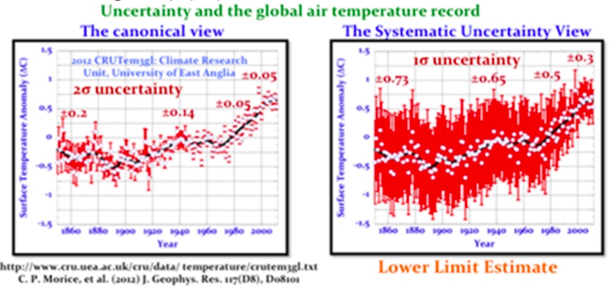
The uncertainty bars for the right hand image reflect a 0.7 to 0.3, SST to land surface ratio of systematic errors. I assume this reflects the ocean 70% surface to the land 30% surface. Bucket and engine-intake errors constitute the SST uncertainty prior to 1990. Over the same time interval the systematic air temperature error of the PRT/CRS sensor package constitute the uncertainty in land-surface temperatures. Floating buoys made a partial contribution (0.25 fraction) to the uncertainty in SST between 1980-1990.
After 1990 uncertainty bars are further steadily reduced, reflecting the increased contribution and smaller errors of Max-Min Temperature System or MMTS on land and floating buoy sea surface sensors.
The right image and the associated numbers are likely more accurate based on actual knowledge than the values in the left hand image. There is a progression of the rate of magnitude of the error values and actual temperature. The right hand revised uncertainty bars represent non-normal systematic error so that the air temperature mean trend loses any status as the most probable trend.
Instrumental Resolution defines the Measurement Detection Limit
Best-case historical 19th and 20th century LiG thermometer with 1º C graduations is +/-0.25º to 0.5º C.
The next slide shows Berkeley Earth global averaged air temperature trend with +/- 2 sigma uncertainty limits in gray.
The time wise +/- 2 sigma instrumental resolution is in red. The blue is a compilation of the best resolution limits of the historical temperature sensors that were used to calculate global resolution limits.
Claims of actual historical instrumentation resolution
The graphic below shows that during the years 1800-1860, the published global uncertainty limits of field meteorological temperatures somehow equals the accuracy of the best possible laboratory conditions that were obtained. After about 1860 through 2000, the published resolution is smaller than the detection/resolution limits of the instruments themselves.

From at least 1860, accuracy has been conjured out of thin air. This is shocking to me but not really surprising when contemplating present day global warming prestidigitations being regularly foisted on us.
So what is it – Negligence, Sloppiness or Lies?
Are these published uncertainties at all credible? Any of us that are field engineers and experimental scientists have to be incredulous. Folks compiling the global instrumental record seem to have completely neglected an experimental limit more basic than systematic measurement error, that is, the detection limits of their instruments. Resolution limits and systematic measurement error produced by the instrument itself constitute the lower limits of uncertainty. But many “consensus” climate scientists seem to have neglected all of the error sources.
These folks seem to have no idea about how to make measurements and seem to have never struggled with using instruments in a field setting. There is no other rational explanation for that sort of negligence than a profound ignorance of experimental methods. The uncertainty estimate developed in this discussion shows that the rate or magnitude of change in global air temperature since 1850 cannot be known within +/- 1º C prior to 1980 and within +/- 0.6º C after 1990 at the 95% confidence interval. Therefor the rate of temperature change within those limits since 1850 is literally unknowable.
Climate Claims
“Unprecedented” warming during any part of the global temperature record cannot be scientifically supported. Claims of the highest air temperature ever, based on even a 0.5º C difference are unsupportable and without any meaning. Finally, there is nothing in the temperature record that warrants a concern for considering an emergency climate action. Except, perhaps, an emergency concerning the apparent competence of AGW-consensus climate scientists.
Other Issues of the Temperature Record
Looking at a marked up copy of the HadCRUT temperature record that I came up with leads to some issues about how the record is being used and abused. Most AGW proponents are generally unwilling to explore some of the natural aspects of the global temperature record.
The following more “realistic” error estimates and some interpretations of cyclical nature of the record are explored.
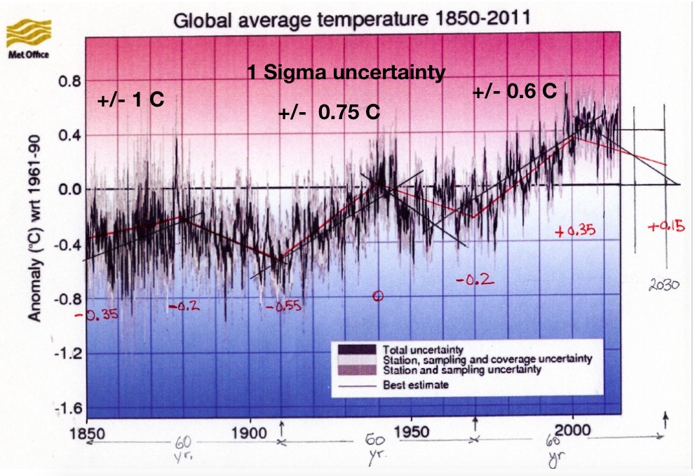
There are two cooling trends clearly seen in this plot, one from the late 1800s until about 1910 and another from about 1941 until about 1970, that are part of a cyclical 60 year pattern. This pattern is related to the Pacific Decadal Oscillation and the Atlantic Multi-decadal Oscillation (PDO/AMO) that are known to be naturally occurring events based on sea surface changes in both of those ocean basins. Some scientists were trying to find instrument improvement causes of the 1940 to 1970 cooling period while indeed it was really a natural phenomenon that can be ascertained from the data.
Now let’s discuss Urban Heat Island effect. This is probably what caused the roughly 0.5º C of added temperature from around 1940 until 2000. The next image shows UHI effects in California for various sizes of populations in counties of that state. Look at the middle plot for counties of 100,000 to 1 million people. About 0.5º C temperature increase especially during that late 20th century period but not any increase for counties of less than 100,000 people. 
You can see by picking temperature data from counties with more than 1 million people you might see a need to predict very catastrophic outcomes. In fact if temperatures are measured only in rural or completely uninhabited areas, only natural fingerprints can be clearly seen.
So there is some slight human caused temperature rise seen late in the last century but mostly from heat producing infrastructure and poorly sited weather stations in the center of large urban settings. But not very likely from human CO2 emissions. This very tiny increase in temperature over the past 70 years of about 0.8º C is lost in the noise even if it could be pinned on humans. The uncertainty of this change could make the increase turn out to be much less than that. When alarmists claim that temperature increases will soon be 4º C it becomes incredible with no scientific basis.
A Local USCRN Station Record – Jornada Range
Even the Berkeley folks noted that USCRN sensors have a resolution of 0.02º C and looking at the measurement methodology we would expect very good accuracy. Here is data from the local USCRN station that is at the Jornada Experiment Range which is north-east of town and mostly outside of the Las Cruces city limit.

Look at the minus 2º C trend line for the 2007 to 2016 record. This shows no warming here in southern NM so my question is, what is happening to the globe in the past few decades? Is it still warming or is it also now beginning to cool?

Other Regional Temperature Indicators
Using raw data from the Western Regional Climate Center I have plotted and analyzed data over the full term of the collection of that data (sometimes up to a hundred years long) with some analysis that I started in about 2006 when I became interested in climate issues.
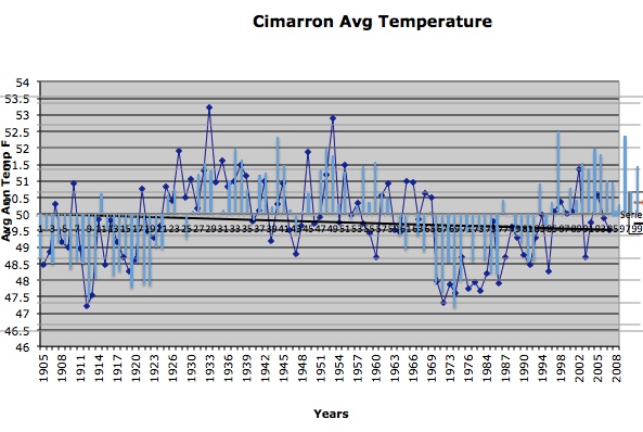
This data came from stations mostly in New Mexico with Cimarron, NM as a bell-weather site since it was very small village in its early days and has remained small even until the present. You can see that the average annual temperature varies about 6 or 7º F over decadal periods.

I later over-laid the Atlantic Multidecadal Oscillation AMO cycle (bars) on top of the temperature plot when I found that NM temperatures seemed to be influenced by this ocean surface temperature index. The 100 year temperature trend seemed to be slightly cooling for Cimarron (see the slightly descending solid trend line in the plot). Without even overlaying the sine wave trend line through the temperature plot, one can see part of a 30 year cooling trend from 1905 until the mid 20s then a 30 year warming trend until the late 1960s followed by cooling until the 1990s. These temperature fluctuations are natural and clearly do not have any warming or cooling overall bias that can often be seen in temperature data from large population centers.
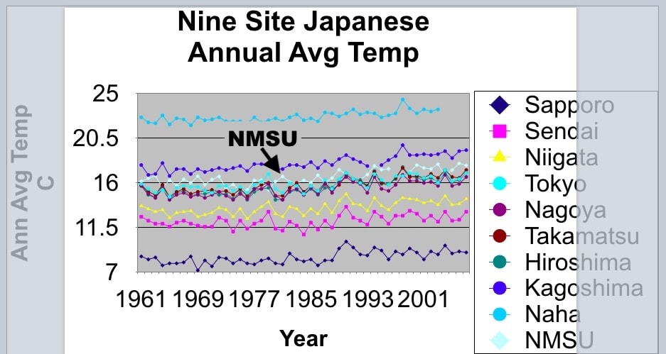
New Mexico temperature throughout the state seem to follow this pattern as seen in the next graphic. With Cimarron in yellow having the coolest temperatures on average as seen below. It’s location in northern NM is the reason for this lower average temperature. NMSU at the top of the plot is the warmest temperature on average and is located in the southern part of the state near El Paso, Texas. 
Finally El Paso temperature for the last part of the 20th century has an apparent warming trend of a little over 1º F over the 60 year period which may be caused by its increasing urbanization and the fact that the site was slowly surrounded by urban sprawl during that period. This warming trend was human caused but probably not global or even regional and found only inside larger cities of the world which cover only about 3% of the land surface of the planet.

Conclusion
Clearly the accuracy of the global temperature record until very recently is poorly defined with large and noisy error bars throughout most of the record. Only by using data from data sensors installed since 2000 can we hope to begin to determine what global temperature trends and values actually are, especially if those global anomalies are 1º C or less. The HadCRUT4 global anomaly temperature record shown four pages back indicates that the past 100+ years of temperature anomaly (toward the warming side) might be just less than 1º C even when human UHI effects, natural effects and all other effects included.
[References Follow the Annex]
Annex to the Global Temperature Error Narrative 9-4-18
This is a short continuation of the above larger error analysis paper to discuss an interesting “out of sync” temperature cycle that lead me to compare temperatures in Japan which sits on the west rim of the Pacific basin with those in New Mexico which is inland from the eastern Pacific rim. ENSO effects such as El Nino and La Nina occur periodically in the broader Pacific Ocean where a pulse of warm water sweeps from Asia toward the South and Central American west coast in a process called El Nino may be implicated in these effects.
First I want to recap some of the concepts from the end of the previous narrative. Temperatures in NM seem to driven by the Atlantic basin and the Atlantic Multidecadal Oscillation (AMO). The AMO index is collected from the Atlantic ocean surface temperatures found from the equator and to the north. PDO effects on North America seem to influence drought and precipitation patterns. When the Pacific is under the influence of an El Nino, Japan seems to “see” La Nina precipitation conditions (cool dry) and vice versa. So here is another out of phase effect seen at opposite edges of the Pacific rim.
This figure shows annual average temperature for Cimarron, NM with the AMO index bar graph over-layed aligned by year. There is very good correlation between them. It is curious that AMO not PDO drives NM temperatures.
The following graph with representative NM annual average temperatures seem to correlate exactly with each other in sequence and amplitude. Note that these annual average temperatures are shown as actual temperatures and not temperature anomalies. Latitude and altitude effects on temperatures are clearly seen in the 10º F temperature difference in cities in the southern versus those northern part of the state. The two larger cities in the group Albuquerque and Las Cruces (NMSU) may be exhibiting a very slight Urban Heat Island (UHI) effect from the 1950s until present.

There does not seem to be any CO2 influence on the annual average temperatures of the small cities of NM (the other 3 plots) over the past 60 years
This lack of CO2 influence seems especially true if you look at the large warm spike for all the plotted cities in 1934 which was a well known “warmest year ever” for almost everywhere in the western US. Another warm year in NM was in 1953. No NM city except Las Cruces has had a recent (1955 to present) warmer temperature than during those two warm years and the spotty data for NMSU (numerous missing years during the whole record) may have just missed “seeing” those two record spikes for the Las Cruces record. All this warming occurred before the growing human CO2 emissions started in the 1960s and with those emissions skyrocketing into the late 90s and on into this century.
How do NM Temperatures Compare to Japanese Temperatures
Basically NMSU temperatures are 180º out of phase with Japanese temperatures. Temperatures of 3 Japanese cities (Tokyo, Nagoya, and Takamatsu) seem to closely match those of Las Cruces but over the classic short periods of 3 to 7 years they are completely opposite in trend.
This longitudinal phasing of temperature effects may be something that Judith Curry has discussed in the “Stadium Wave” theory.
https://judithcurry.com/2013/10/10/the-stadium-wave/
There seems to be an out of phase effect of several ocean temperature indexes such as the PDO and the AMO that looks like a wave found with cheering crowds at a football stadium which is a wave of people standing and raising their arms that travels around the stadium but in this case travels around the globe. At the sports arena, it may take only a few minutes to completely travel around the stadium while the Curry Global Stadium Wave may take several years.
Annex Conclusions
I found this cross basin temperature difference by accident when I compared my NM temperature data with data that I had collected on Japan. I quickly noticed the 3 to 7 year short term temperature swings of the data in NM and Japan and that those short up and down cycles occurred at all sites in NM in sync as well as in Japan among the regional stations. The regional site temperatures had a similar pattern to all the sites in the region be it NM or Japan.
But when I added the NMSU data in degrees centigrade to the collected Japanese data, I quickly saw that those swings though similar were exactly out of phase.
What causes the stadium wave effect? Some sort of ocean currents and ENSO effects? Coriolis driven winds? Does it proceed west to east like the Jet Stream and the Gulf Stream? We can probably safely say that it is fundamentally caused by changing solar radiative effects along with a spinning earth and probably is not caused at all by CO2.
References
[1] JCGM, Evaluation of measurement data — Guide to the expression of uncertainty in measurement 100:2008, Bureau International des Poids et Mesures: Sevres, France.
[2] Frank, P., et al., Determination of ligand binding constants for the iron-molybdenum cofactor of nitrogenase: monomers, multimers, and cooperative behavior. J. Biol. Inorg. Chem., 2001. 6(7): p. 683-697.
[3] Frank, P. and K.O. Hodgson, Cooperativity and intermediates in the equilibrium reactions of Fe(II,III) with ethanethiolate in N-methylformamide solution. J. Biol. Inorg. Chem., 2005. 10(4): p. 373-382.
[4] Hinkley, N., et al., An Atomic Clock with 10-18 Instability. Science, 2013. 341(p. 1215-1218.
[5] Parker, D.E., et al., Interdecadal changes of surface temperature since the late nineteenth century. J. Geophys. Res., 1994. 99(D7): p. 14373-14399.
[6] Quayle, R.G., et al., Effects of Recent Thermometer Changes in the Cooperative Station Network. Bull. Amer. Met. Soc., 1991. 72(11): p. 1718-1723; doi: 10.1175/1520-0477(1991)072<1718:EORTCI>2.0.CO;2.
[7] Hubbard, K.G., X. Lin, and C.B. Baker, On the USCRN Temperature system. J. Atmos. Ocean. Technol., 2005. 22(p. 1095-1101.
[8] van der Meulen, J.P. and T. Brandsma, Thermometer screen intercomparison in De Bilt (The Netherlands), Part I: Understanding the weather-dependent temperature differences). International Journal of Climatology, 2008. 28(3): p. 371-387.
[9] Barnett, A., D.B. Hatton, and D.W. Jones, Recent Changes in Thermometer Screen Design and Their Impact in Instruments and Observing Methods WMO Report No. 66, J. Kruus, Editor. 1998, World Meteorlogical Organization: Geneva.
[10] Lin, X., K.G. Hubbard, and C.B. Baker, Surface Air Temperature Records Biased by Snow-Covered Surface. Int. J. Climatol., 2005. 25(p. 1223-1236; doi: 10.1002/joc.1184.
[11] Hubbard, K.G. and X. Lin, Realtime data filtering models for air temperature measurements. Geophys. Res. Lett., 2002. 29(10): p. 1425 1-4; doi: 10.1029/2001GL013191.
[12] Huwald, H., et al., Albedo effect on radiative errors in air temperature measurements. Water Resorces Res., 2009. 45(p. W08431; 1-13.
[13] Menne, M.J. and C.N. Williams, Homogenization of Temperature Series via Pairwise Comparisons. J. Climate, 2009. 22(7): p. 1700-1717.
[14] Briffa, K.R. and P.D. Jones, Global surface air temperature variations during the twentieth century: Part 2 , implications for large-scale high-frequency palaeoclimatic studies. The Holocene, 1993. 3(1): p. 77-88.
[15] Hansen, J. and S. Lebedeff, Global Trends of Measured Surface Air Temperature. J. Geophys. Res., 1987. 92(D11): p. 13345-13372.
[16] Brohan, P., et al., Uncertainty estimates in regional and global observed temperature changes: A new data set from 1850. J. Geophys. Res., 2006. 111(p. D12106 1-21; doi:10.1029/2005JD006548; see http://www.cru.uea.ac.uk/cru/info/warming/.
[17] Karl, T.R., et al., The Recent Climate Record: What it Can and Cannot Tell Us. Rev. Geophys., 1989. 27(3): p. 405-430.
[18] Hubbard, K.G., X. Lin, and E.A. Walter-Shea, The Effectiveness of the ASOS, MMTS, Gill, and CRS Air Temperature Radiation Shields. J. Atmos. Oceanic Technol., 2001. 18(6): p. 851-864.
[19] MacHattie, L.B., Radiation Screens for Air Temperature Measurement. Ecology, 1965. 46(4): p. 533-538.
[20] Rüedi, I., WMO Guide to Meteorological Instruments and Methods of Observation: WMO-8 Part I: Measurement of Meteorological Variables, 7th Ed., Chapter 1. 2006, World Meteorological Organization: Geneva.
[21] Berry, D.I. and E.C. Kent, Air–Sea fluxes from ICOADS: the construction of a new gridded dataset with uncertainty estimates. International Journal of Climatology, 2011: p. 987-1001.
[22] Challenor, P.G. and D.J.T. Carter, On the Accuracy of Monthly Means. J. Atmos. Oceanic Technol., 1994. 11(5): p. 1425-1430.
[23] Kent, E.C. and D.I. Berry, Quantifying random measurement errors in Voluntary Observing Ships’ meteorological observations. Int. J. Climatol., 2005. 25(7): p. 843-856; doi: 10.1002/joc.1167.
[24] Kent, E.C. and P.G. Challenor, Toward Estimating Climatic Trends in SST. Part II: Random Errors. Journal of Atmospheric and Oceanic Technology, 2006. 23(3): p. 476-486.
[25] Kent, E.C., et al., The Accuracy of Voluntary Observing Ships’ Meteorological Observations-Results of the VSOP-NA. J. Atmos. Oceanic Technol., 1993. 10(4): p. 591-608.
[26] Rayner, N.A., et al., Global analyses of sea surface temperature, sea ice, and night marine air temperature since the late nineteenth century. Journal of Geophysical Research-Atmospheres, 2003. 108(D14).
[27] Emery, W.J. and D. Baldwin. In situ calibration of satellite sea surface temperature. in Geoscience and Remote Sensing Symposium, 1999. IGARSS ’99 Proceedings. IEEE 1999 International. 1999.
[28] Emery, W.J., et al., Accuracy of in situ sea surface temperatures used to calibrate infrared satellite measurements. J. Geophys. Res., 2001. 106(C2): p. 2387-2405.
[29] Woodruff, S.D., et al., The Evolving SST Record from ICOADS, in Climate Variability and Extremes during the Past 100 Years, S. Brönnimann, et al. eds, 2007, Springer: Netherlands, pp. 65-83.
[30] Brooks, C.F., Observing Water-Surface Temperatures at Sea. Monthly Weather Review, 1926. 54(6): p. 241-253.
[31] Saur, J.F.T., A Study of the Quality of Sea Water Temperatures Reported in Logs of Ships’ Weather Observations. J. Appl. Meteorol., 1963. 2(3): p. 417-425.
[32] Barnett, T.P., Long-Term Trends in Surface Temperature over the Oceans. Monthly Weather Review, 1984. 112(2): p. 303-312.
[33] Anderson, E.R., Expendable bathythermograph (XBT) accuracy studies; NOSC TR 550 1980, Naval Ocean Systems Center: San Diego, CA. p. 201.
[34] Bralove, A.L. and E.I. Williams Jr., A Study of the Errors of the Bathythermograph 1952, National Scientific Laboratories, Inc.: Washington, DC.
[35] Hazelworth, J.B., Quantitative Analysis of Some Bathythermograph Errors 1966, U.S. Naval Oceanographic Office Washington DC.
[36] Kennedy, J.J., R.O. Smith, and N.A. Rayner, Using AATSR data to assess the quality of in situ sea-surface temperature observations for climate studies. Remote Sensing of Environment, 2012. 116(0): p. 79-92.
[37] Hadfield, R.E., et al., On the accuracy of North Atlantic temperature and heat storage fields from Argo. J. Geophys. Res.: Oceans, 2007. 112(C1): p. C01009.
[38] Castro, S.L., G.A. Wick, and W.J. Emery, Evaluation of the relative performance of sea surface temperature measurements from different types of drifting and moored buoys using satellite-derived reference products. J. Geophys. Res.: Oceans, 2012. 117(C2): p. C02029.
[39] Frank, P., Uncertainty in the Global Average Surface Air Temperature Index: A Representative Lower Limit. Energy & Environment, 2010. 21(8): p. 969-989.
[40] Frank, P., Imposed and Neglected Uncertainty in the Global Average Surface Air Temperature Index. Energy & Environment, 2011. 22(4): p. 407-424.
[41] Hansen, J., et al., GISS analysis of surface temperature change. J. Geophys. Res., 1999. 104(D24): p. 30997–31022.
[42] Hansen, J., et al., Global Surface Temperature Change. Rev. Geophys., 2010. 48(4): p. RG4004 1-29.
[43] Jones, P.D., et al., Surface Air Temperature and its Changes Over the Past 150 Years. Rev. Geophys., 1999. 37(2): p. 173-199.
[44] Jones, P.D. and T.M.L. Wigley, Corrections to pre-1941 SST measurements for studies of long-term changes in SSTs, in Proc. Int. COADS Workshop, H.F. Diaz, K. Wolter, and S.D. Woodruff, Editors. 1992, NOAA Environmental Research Laboratories: Boulder, CO. p. 227–237.
[45] Jones, P.D. and T.M.L. Wigley, Estimation of global temperature trends: what’s important and what isn’t. Climatic Change, 2010. 100(1): p. 59-69.
[46] Jones, P.D., T.M.L. Wigley, and P.B. Wright, Global temperature variations between 1861 and 1984. Nature, 1986. 322(6078): p. 430-434.
[47] Emery, W.J. and R.E. Thomson, Data Analysis Methods in Physical Oceanography. 2nd ed. 2004, Amsterdam: Elsevier.
[48] Frank, P., Negligence, Non-Science, and Consensus Climatology. Energy & Environment, 2015. 26(3): p. 391-416.
[49] Folland, C.K., et al., Global Temperature Change and its Uncertainties Since 1861. Geophys. Res. Lett., 2001. 28(13): p. 2621-2624.
______________________