
By Robert W. Endlich
Author’s Note: This is Part TWO of a multiple post topic. Figure numbers remain consecutive across the four parts of the post.
Part ONE is here.
Part THREEis here.
Part FOUR is here.
Presentation is here.
THE “SOLAR CONSTANT” IS NOW VARIABLE? YES, IT IS TRUE!
When I was an Undergraduate in Basic Meteorology, 1963-64 at Texas A&M, and Graduate Student, 1967-69, Penn State, we learned that the “Solar Constant” was 2 calories/cm**2/sec. But sometimes we used 1.94 cal/cm**2/sec ….in the CGS, the Centimeter-Gram-Second system of measurements.
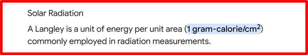
Sometimes we used 2 Langleys per second…after this definition, in terms of Langleys, graphic below.
In 2024’s retrospect, the 1960s were seemingly in the Dark Ages of academic endeavor.
Figures 4 and 5 below will help explain further developments.
Figure 4 is a time series of Total Solar Irradiance from the 1600s to 2015. The ordinate is in Watts/meter**2, in black, with the present estimate of the solar constant, in green, from Kopp and Lean, 2011, as 1.951 Langleys per second.
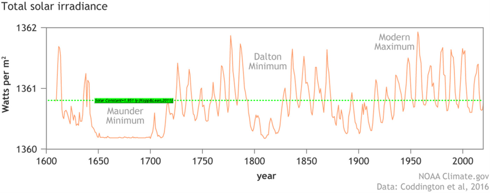
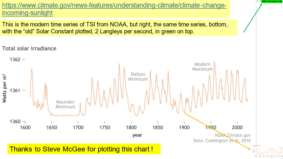
CASF member Steve McGee kindly plotted comparisons between the 1960s definition of the solar constant, 2 Langleys per second, with a modern (2016) definition at 1.951 Langleys per second, in green, in Figure 4 above, and separately in Figure 5, below.
Look carefully at Figure 5, because there are two graphics there. While most of the plot, especially the time series in orange resembles the time series of Figure 4, there are orange and green arrows which point to another graphic on the right, with an expanded ordinate range which shows the 1600-2015 time series at the bottom, and the old 1960s version of the solar constant plotted as 2 Langleys per second on the right side.
I attribute much of the credit for the discovery that the ‘solar constant’ is not constant at all, and that there was, and is, a causal relationship between low solar output and the very cold temperatures in the depth of the Little Ice Age, publication of which came in the 1970s. Specifically, John Eddy’s paper in Science, 19 Jun 1976, “The Maunder Minimum”, is in my opinion, a detective story of sorts. This paper’s conclusion delves into the coincidence of Maunder’s “prolonged solar minimum” with the coldest excursion of temperatures, the Little Ice Age…and “possible relations between the sun and terrestrial climate”
GEOLOGIC PROCESSES AND SEA LEVEL
This topic is vast and could, and does, cover chapters in physical geology texts. Below are just a few elements to touch on here.
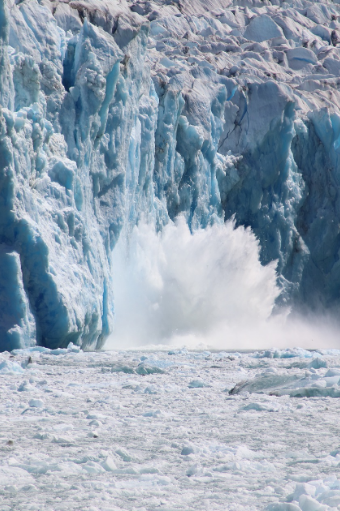
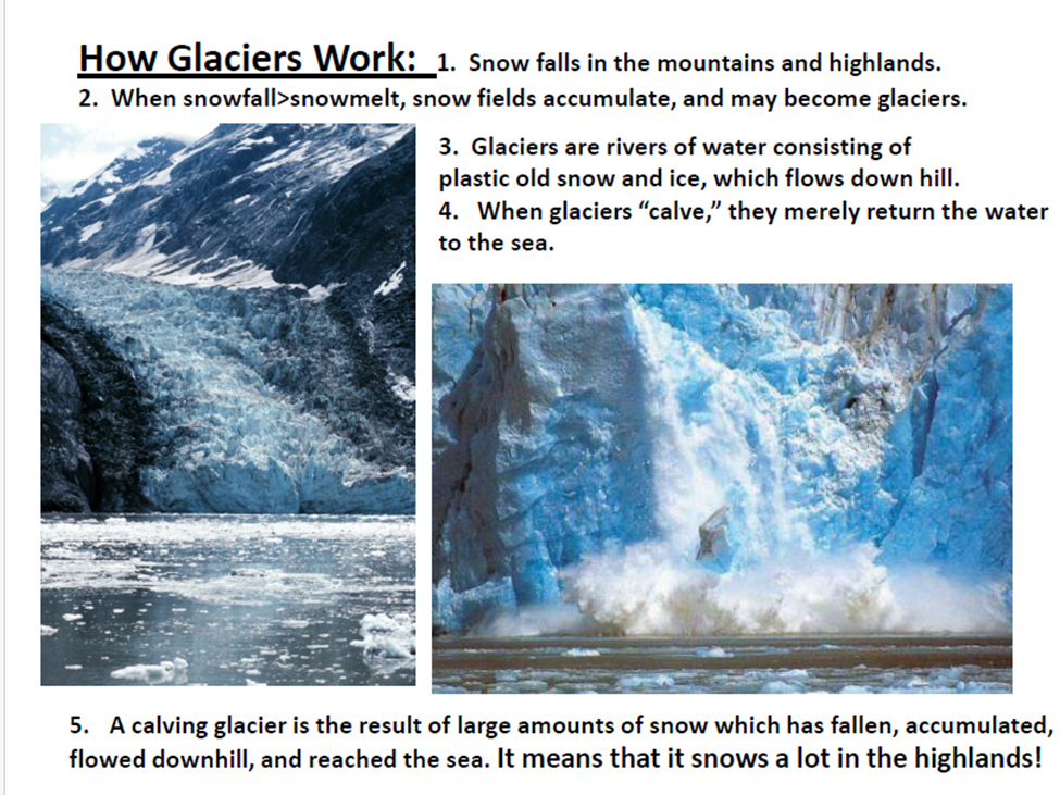
CALVING GLACIERS
Calving glaciers are sometimes given as evidence for human-caused CO2-fueled global warming. Figure 6 shows how this is not the case, calving glaciers can and do occur when global temperatures are cooling!
GROUNDWATER EXTRACTION FROM UNCONSOLIDATED AND SEMI-CONSOLIDATED SEDIMENTS
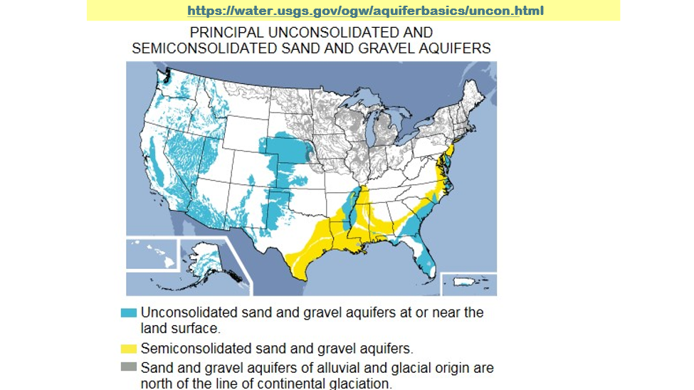
In the Continental US, the Atlantic and Gulf Coastal Plains extend from Long Island, NY, generally southward to eastern NC, and thereafter, southwestward to near Del Rio, TX. These are the blue and yellow areas eastward from the Rio Grande of Texas to Long Island in Fig 7 below.
Unconsolidated and semi-consolidated sediments are formations of sand, silt, clay and minor carbonate rocks that typically are aquifers, that is, they contain water in the interstitial spaces between the particles or grains. Especially when ground water is extracted by us humans, this type of geological formation is called an aquifer.
Figure 7 below, from the presentation graphics, is a map from the US Geological Survey showing the areal extent of the unconsolidated (in blue) and semi-consolidated (in yellow) sand, mud and gravel sedimentary formations. Many of these areas have high population densities. When uncontrolled groundwater pumping occurs, mass is removed from the interstitial spaces between the sediment’s grains. With water removed from these spaces, the formations permanently collapse. When this process is not controlled, but continues unabated, significant and harmful ground subsidence results.
TIDE GAGES RECORD WATER LEVELS, BUT THEY CAN’T THINK FOR US
We will get deeper into the subject of Tide Gages later. But, to introduce this, we need to say that tide gages use a float similar in principle to that of the toilet tank float. When the toilet is flushed, the water in the tank falls and the float mechanism sends a mechanical signal to open the water valve. When water again fills the tank, the rising float sends a signal that the tank is full, and it turns the water valve off.
When sea levels rise, tide gages indicate how much the sea level rises because the rising water lifts the float in the tide gage, signaling a higher water level. But there are many areas where ground water pumping has led to significant land subsidence where the tide gage is located. By itself, the tide gage cannot tell the difference between ground water pumping and sea level rise.
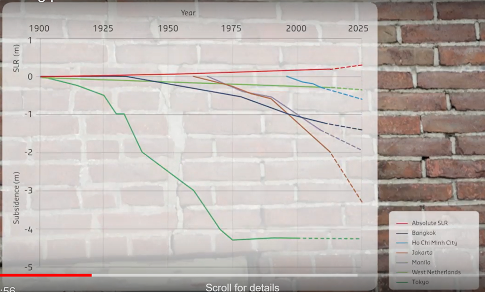
This has led to cries of accelerated sea level rise by global warming Alarmists. This video, “Subsidence, a Growing Problem,” shows a graphic displaying sea level rise since 1900, and the change in ground level, the subsidence, of these cities of the world: Bangkok, Saigon aka Ho Chi Minh City, Jakarta, Manila, the west Netherlands, and Tokyo. Note well, the displayed rates of subsidence are many times the rate of sea level rise!
Evidence neither Earth’s surface nor the levels of the seas are static:
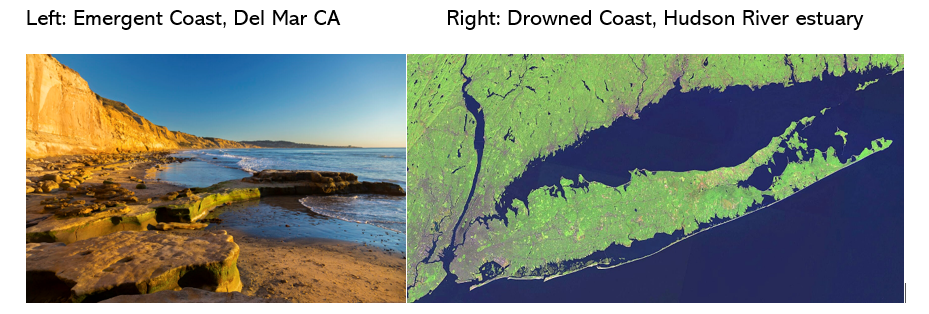
From Figure 9 below: on the left shows the West Coast of the USA, Del Mar, CA, near San Diego, where the coastline is emerging from the Pacific Ocean at a significant rate. There is almost no sandy beach, and almost vertical cliffs emerge directly from the Pacific. The Pacific Coast Ranges of mountains are very close to the Pacific.
On the right is a satellite image of the East Coast, where New York’s Hudson River meets the Atlantic Ocean, and all of Long Island, NY. At the last glacial maximum, when sea levels were some 400 ft lower than today, the Hudson carved the Hudson Canyon, eroding a huge gash in what we now call the Continental Shelf.
Today, rather than the Hudson emptying directly into the Atlantic as it did during the Wisconsin Ice Age, this entire area has been flooded or “drowned” by the rising sea level from the melting of the continental glaciers of the last ice age, the Wisconsin Ice Age as it is known in North America. As a consequence, high tides now extend upriver to Troy, NY, 157 miles from the Atlantic.
In summary, the solar constant is not actually a constant and varies with time. Also, sea level is complicated by the fact that it not only rises and falls, but the sea shores frequently subside and the tide gages combine the effects of subsidence along with the rise or fall of sea level.
In Part THREE, I will disprove claims made by NPR, PNAS, and other mainstream outlets that the ice at the poles is “rapidly melting.”